Introduction
In the rapidly evolving world of machine learning (ML), data scientists and ML engineers face a common challenge: efficiently managing and reusing features across multiple models. Feature engineering, a crucial step in the ML development process, can be time-consuming and repetitive, leading to delays in model deployment and reduced productivity. This is where the concept of an ML Feature Store comes into play.
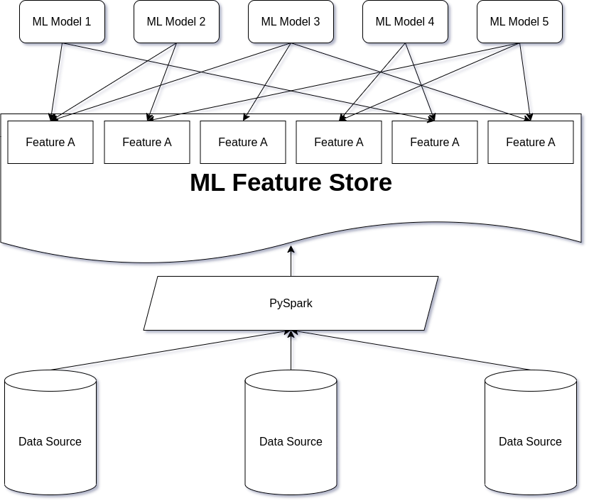
An ML Feature Store is a centralized repository that allows teams to store, manage, and access features used in ML models. It acts as a single source of truth for feature data, enabling different ML models to reuse the same features without the need for :wredundant feature engineering efforts. By providing a unified interface for storing and retrieving features, a Feature Store streamlines the ML development process and significantly reduces the time-to-market for new models.
One of the key benefits of a Feature Store is its ability to promote feature reuse across multiple models. Instead of each model having its own siloed feature set, a Feature Store allows features to be shared and reused by different models. This not only saves time and effort in feature engineering but also ensures consistency and maintainability across the ML ecosystem.

Feature Store based on customers behaviour
In the realm of customer interaction-based features, these features are typically aggregates of various interactions, such as the number of logins, clicks, or average spending from a credit card, calculated over different time periods and grouped by specific categories.
For instance, a Feature Store can be used to create features like the amount of logins in the mobile category for the last three months or the average spending in the grocery category from a credit card with the type “Credit Card.” These features provide valuable insights into customer behavior and preferences, which can be leveraged by machine learning models to make informed predictions and drive personalized experiences.
In the following sections, we will delve deeper into the specific use case of creating features based on customer interactions using PySpark.
Technical introduction
One might say that creating such a feature store requires working with window functions because of the time component, but time intervals can easily be encoded as group columns, so the task is just to calculate different aggregates (sum, count, average, etc.) over different group combinations. For example, if we have a timeline column, say login_date, and we need to calculate aggregates for the last week, month, and six months, it is easy to create additional columns with flags to avoid window functions:
from pyspark.sql import functions as F

data_with_flags = (
  data
  .withColumn(
    "last_week_flag",
    (F.datediff(F.current_date(), F.col("login_date")) <= F.lit(7))
  )
  .withColumn(
    "last_month_flag",
    (F.datediff(F.current_date(), F.col("login_date")) <= F.lit(30.5))
  )
  .withColumn(
    "last_six_month_flag",
    (F.datediff(F.current_date(), F.col("login_date")) <= F.lit(30.5 * 6))
  )
)
So, the task of calculation of a single batch of the Feture Store table can be transformed into the generic task of aggregations over multiple groups. Let’s use H2O benchmark dataset as an example:
from pyspark.sql import SparkSession

spark = (
    SparkSession.builder
    .master("local[*]")
    .getOrCreate()
)

schema = T.StructType.fromJson(
    {'type': 'struct',
     'fields': [{'name': 'id1',
       'type': 'string',
       'nullable': True,
       'metadata': {}},
      {'name': 'id2', 'type': 'string', 'nullable': True, 'metadata': {}},
      {'name': 'id3', 'type': 'string', 'nullable': True, 'metadata': {}},
      {'name': 'id4', 'type': 'integer', 'nullable': True, 'metadata': {}},
      {'name': 'id5', 'type': 'integer', 'nullable': True, 'metadata': {}},
      {'name': 'id6', 'type': 'integer', 'nullable': True, 'metadata': {}},
      {'name': 'v1', 'type': 'integer', 'nullable': True, 'metadata': {}},
      {'name': 'v2', 'type': 'integer', 'nullable': True, 'metadata': {}},
      {'name': 'v3', 'type': 'double', 'nullable': True, 'metadata': {}}]}
)

data = (
  spark.read
  .option("header", "true")
  .schema(schema)
  .csv("data/G1_1e6_1e6_10_0.csv")
)
data.show()
Result:
+-----+-----+------------+---+---+-----+---+---+--------+
|  id1|  id2|         id3|id4|id5|  id6| v1| v2|      v3|
+-----+-----+------------+---+---+-----+---+---+--------+
|id008|id006|id0000098213|  6|  1| 9802|  1|  9|34.51913|
|id007|id003|id0000022646|  8|  1|20228|  1|  4|64.95154|
|id008|id004|id0000083470|  1|  6| 2125|  1|  8|43.23634|
|id009|id006|id0000051855|  5|  8|41429|  1| 12|27.36826|
|id005|id007|id0000074629| 10|  1|71480|  2| 15|65.04233|
|id001|id009|id0000045958|  6|  2|30060|  5|  8|16.57359|
|id009|id008|id0000060869| 10| 10|95489|  4|  8|60.78273|
|id010|id010|id0000015471|  3|  2|53762|  5| 11|40.72817|
|id008|id009|id0000032117| 10|  7|37774|  4|  2| 7.48368|
|id006|id001|id0000064092|  4|  5|64203|  1| 15|79.79128|
|id001|id001|id0000041819|  3|  3|91110|  2| 11|34.33383|
|id005|id004|id0000097955|  3|  6|95321|  5|  7|32.20545|
|id009|id005|id0000004865|  6| 10|54982|  3|  8| 3.07528|
|id008|id009|id0000060610|  8| 10|31843|  1|  8|37.05268|
|id009|id009|id0000008902|  8|  9| 9394|  4| 13|23.04208|
|id006|id004|id0000044586|  6|  6| 5279|  2|  6|49.30788|
|id007|id007|id0000015887| 10|  1| 2987|  2|  1|66.90033|
|id007|id003|id0000039177|  2|  3|85798|  4|  2|31.13281|
|id002|id004|id0000066644|  9|  1|57709|  1| 12|53.35556|
|id006|id003|id0000064335|  7|  5|38365|  2|  7|59.54201|
+-----+-----+------------+---+---+-----+---+---+--------+
The entire data set has 1,000,000 rows. Here we have the column id3 which is a string and has ~100,000 unique values. This column represents a unique key, for example a customer id. The columns id1, id2, id4, id5 have 10 unique but independent values and will represent our grouping keys, like time interval flag and different categories.
To reproduce my experiment, you can use the farsante library, which contains effective H2O dataset generators written in Rust. See the documentation for details. I used the rust cli api of farsante and the following commands to genrate this dataset:
cargo build --release
cd target/release
./farsante --n 1000000 --k 10
GroupBy + Pivot approach
Our goal is to take our initial data with 9 columns and 1,000,000 rows and create a feature table with 121 columns and 100,000 rows. In this case, 121 columns contains
- id column (
"id3") count("*"), sum("v2"), avg("v3")for all unique values of column id1 (3 * 10 = 30 columns)count("*"), sum("v2"), avg("v3")for all unique values of col id2 (3 * 10 = 30 cols)count("*"), sum("v2"), avg("v3")for all unique values of col id4 (3 * 10 = 30 cols)count("*"), sum("v2"), avg("v3")for all unique values of col id5 (3 * 10 = 30 cols)
120 + 1 columns in total. We will only touch on the simplest case, without touching on the topic of combinations of group values. But as you will see, our code is easily extendable to this case. We need to create a structure with columns that contain values of group keys in their names. The most obvious way to do this is to simply use groupBy + pivot in PySpark. But since we are talking about a production-like pipeline, the output schema of our table should not depend on the input data, so we need to fix the values of the group keys before computing anything. In our example, we can infer these values, but in production, of course, it is strongly recommended to fix these values at the level of pipeline configuration files. Otherwise, you could easily shoot yourself in the foot one day when a new group key comes along and breaks your table schema.
groups = {
    "id1": [d[0] for d in data.select(F.col("id1")).distinct().collect()],
    "id2": [d[0] for d in data.select(F.col("id2")).distinct().collect()],
    "id4": [d[0] for d in data.select(F.col("id4")).distinct().collect()],
    "id5": [d[0] for d in data.select(F.col("id5")).distinct().collect()],
}

PRIMARY_KEY = "id3"
By using this structure it is easy to write the naive groupBy-pivot version:
from functools import reduce

def naive_fs(data, groups):
    pre_result = []
    for grp_col in groups.keys():
        pre_result.append(
            data
            .groupBy(PRIMARY_KEY)
            .pivot(grp_col, groups[grp_col])
            .agg(
                F.count("v1").alias(f"_valof_{grp_col}_count_v1"),
                F.sum("v2").alias(f"valof_{grp_col}_sum_v2"),
                F.mean("v3").alias(f"valof_{grp_col}_avg_v3"),
            )
        )
    return reduce(lambda a, b: a.join(b, on=[PRIMARY_KEY], how="left"), pre_result)
Let’s see how fast it produce our tiny dataset with one million of rows:
%%time
naive_fs(data, groups).write.mode("overwrite").parquet("tmp/naive_output")
Results (each run means a full restart of SparkSession to avoid getting confusing results due to disk hashing or AQE optimizations):
- Run N1:
CPU times: user 44.5 ms, sys: 9.43 ms, total: 53.9 ms
Wall time: 21.8 s
- Run N2:
CPU times: user 41.1 ms, sys: 11.3 ms, total: 52.4 ms
Wall time: 20.2 s
- Run N3:
CPU times: user 49.3 ms, sys: 7.53 ms, total: 56.8 ms
Wall time: 21.8 s
Spark Plan analysis
Opening a Spark plan shows me that in this case Spark actually does three sort-merge joins. Trying the same code but with 10 million rows dataset will get stuck and fail with Java heap space (on distributed cluster it will transform into huge data spill and most likely fail due to disk space or even it may brake the whole cluster if it is not protected from disk overflow).
Case-when approach
Another approach is to use the CASE-WHEN approach. For example, to compute the count(*) over some group, we can avoid using groupBy at all, just because the count of rows related to some value val of a group key is just a sum over a CASE-WHEN expression like this: F.sum(F.when(F.col("grp_key") == F.lit(val), F.lit(1)).otherwise(F.lit(0))). In this case, we use case-when to return 1 for all rows related to the group and zero otherwise. The sum over such a result is obviously equal to the number of rows related to the value of the group. To calculate sum we can use the value of the sum column for rows related to the group and zero otherwise. To calculate the average, we need to replace unrelated rows with null, because the built-in Spark averaging function ignores null. You can check the documentation to understand how to calculate other types of aggregates.
Let’s write the code, that generate our aggragations for H2O dataset:
def case_when_fs(data, groups):
    cols_list = []
    for grp_col, values in groups.items():
        for val in values:
            cond = F.col(grp_col) == F.lit(val)
            cols_list.append(
                F.sum(F.when(cond, F.lit(1)).otherwise(F.lit(0))).alias(f"{val}_valof_{grp_col}_count_v1")
            )
            cols_list.append(
                F.sum(F.when(cond, F.col("v2")).otherwise(F.lit(0))).alias(f"{val}_valof_{grp_col}_sum_v2")
            )
            cols_list.append(
                F.mean(F.when(cond, F.col("v2")).otherwise(F.lit(None))).alias(f"{val}_valof_{grp_col}_avg_v3")
            )
    return data.groupby(PRIMARY_KEY).agg(*cols_list)
We will run the same test with write for that approach:
%%time
case_when_fs(data, groups).write.mode("overwrite").parquet("tmp/case_when_output")
Results:
- Run N1:
CPU times: user 157 ms, sys: 40.5 ms, total: 198 ms
Wall time: 13.9 s
- Run N2:
CPU times: user 176 ms, sys: 35.6 ms, total: 211 ms
Wall time: 14.3 s
- Run N3:
CPU times: user 192 ms, sys: 41.3 ms, total: 233 ms
Wall time: 16.9 s
Spark Plan analysis
In this case, there are no sort-merge-join operations in the plan. The calculation is almost x1.5 faster. Also, this code will work in the case of 10 million rows without errors (out-of-core case) without disk spill and Java heap space errors. Also, this approach give you more prciese control over the variable names, groups combinations, etc.
Conclusion
The described above case is quite specific, but still very offen. And it is a nice example, how engineers can use domain knowledge about keys distribution, required output, etc. to write less generic but more effective code!