TLDR;
I don’t think anyone besides me has considered using Apache DataFusion to write graph algorithms. I still don’t fully understand DataFusion’s place in the world of graphs, but I’d like to share my initial experience with it. Spoiler alert: It’s surprisingly good! In this post, I will explain the weakly connected components problem and its close relationship to the common problem of modern data warehouses (DWHs), namely, identity resolution. I will also describe an algorithm for connected components in a MapReduce paradigm. I consider this to be the algorithm that strikes the best balance between performance and simplicity. Finally, I’ll present my DataFusion-based implementation of the algorithm and the results of toy benchmarks on a graph containing four million nodes and 129 million edges. As always, keep in mind that this post is very opinionated!
Preface
I’m not an experienced Rust developer. I’m just beginning to explore the Apache DataFusion project. Although I am the most active maintainer of the Apache Spark-based project GraphFrames, I cannot say that I am excellent at graph theory or hard computer science. I would describe myself as a curious developer who likes graphs, graph algorithms, and writing code myself (not telling someone or an LLM to write code). I’m not trying to critique any open-source developer, especially the truly cool people who maintain the DataFusion project. Even if something in this post may look like criticism, it actually isn’t. I’m simply sharing my experience as a regular software and programming enthusiast!
Introduction
Connected Components problem
Before we go further let me explain some very basic concepts from the graph theory first. The top level thing is Graph itself. In the simplest case it is just a set of vertices \( \{V\} \) connected by the set of edges \( \{ E \} = (v_i, v_j) | v_i, v_j \in \{ V \} \). Actually graph is just a set of entities and connections between them. As each edge contains two vertices, we may say that one of them is a source and the second is destination. While graphs can be directed, when existing of the edge \( e_{ij} \) does not mean the existing of the edge \( e_{ji} \), for simplicity we will talk further only about undirected graphs. In undirected graphs, as it is clear from the name itself, the edge direction does not matter at all, so edge \( e_{ij} \) is at the same time the edge \( e_{ji} \).
When we have a graph, we may say that two vertices are connected when there is an edge between them. We need also introduce a concept of path. Path is a sequence of vertices so each vertex of it is connected with a previous one. Also we may say that vertex \( v_i \) is reachable from the vertex \( v_j \) if there exists a path between them.
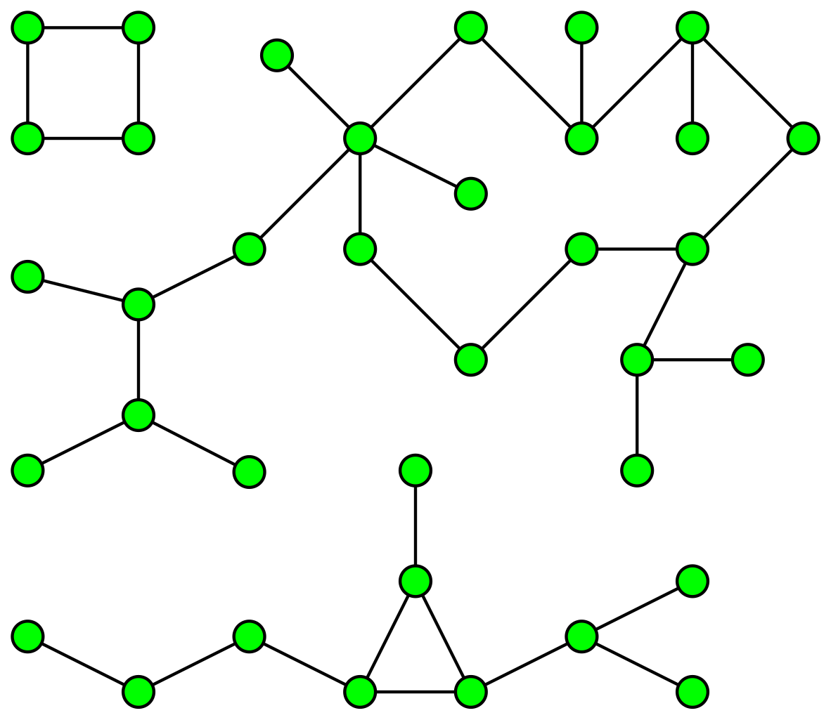
Connected Component of the Graph is a subset of vertices from \( \{ V \} \), where each vertex from this subset is reachable by any other vertex from the same subset.
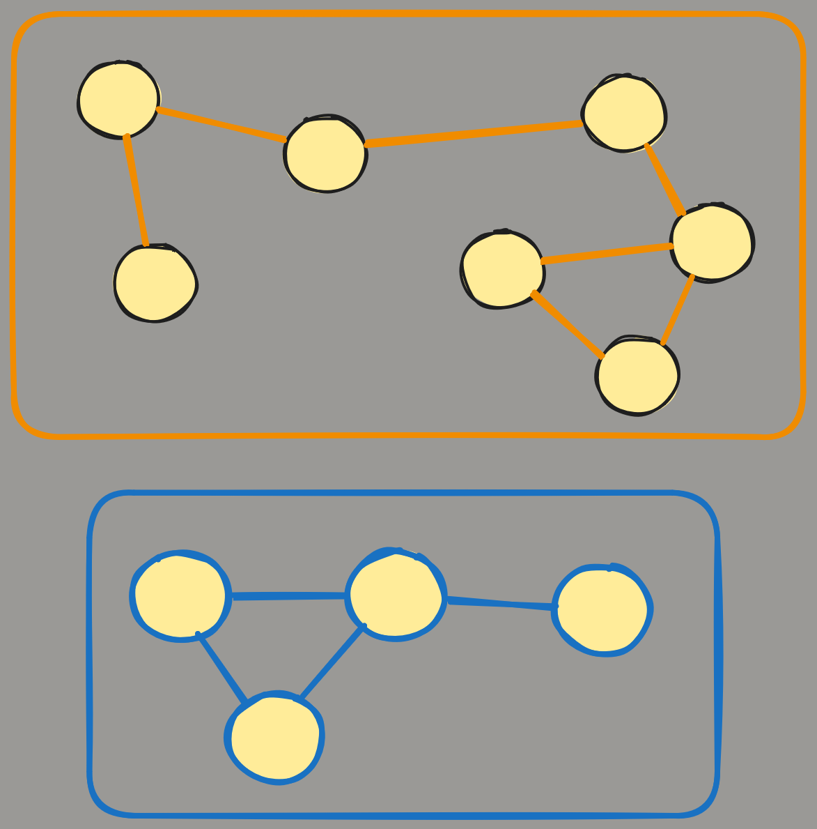
In plain English, Connected Component is a small graph (or the so-called sub-graph) inside a bigger graph. If, for example, the graph has two connected components, we may just say that there are two graphs because each of them is separated from another.
NOTE: For simplicity we are talking here only about undirected graphs. But if the graph is directed, there are actually two different way of defining connected components. One is by ignoring edge direction, so inside each of components every vertex is reachable by all other vertices by the undirected path. And the second, obviously, by respecting edge directions, so each vertex of the component should be reached by directed path from all other vertices of the component. The first definition is known as the Weakly Connected Components problem and the second definition leads us to the Strongly Connected Components problem. In this post we are talking about the weakly connected components because of the link between this problem and the identity resolution problem of the modern DWHs. For simplicity, if further I mention Connected Components, I mean Weakly Connected Components.
Identity resolution problem
While the most of graph problems are quite a specific and regular DWH developer, BI Analyst or Data Engineer rarely face them (outside of the whiteboard coding interview sections), Connected Components is an exception. And the reason is it’s connection to the identity resolution problem.
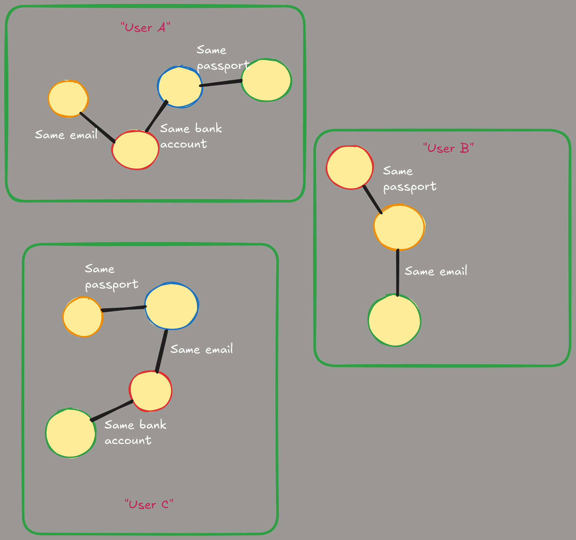
Let’s imagine the very common case. We are a Data Engineer working with a Data Warehouse. Our DWH has a lot of different sources of data. And these sources have their own identity systems. Let’s imagine we are buying data from data brokers or ingesting it from different production systems. In that case it is common that there is no single ID for entities such as, for example, users. All the sources have their own internal IDs (typically some kind of UUIDs) as primary keys. And the problem here is to create the so called “golden row” (or “super-ID”) by matching data from sources using their attributes. For example, source may have partially filled fields like “user_email”, “user_passport”, “bank_account_number”, “mobile_device_id”, etc.
While it may be possible to resolve such a problem in a straight-forward SQL way of sequential joins and null-checks it may be very expensive. Not only from the resources point of view, but from coding view too. The biggest problem is that joins order is non-obvious as well one face a lot of actually not needed joins with a naive implementation. Even on a small-medium sized graphs it will be very hard. And on a real-world scale when sources have terabytes of data it simply won’t work. Especially because order of joins is not obvious, size of dataset may be very different, etc.
At the same time, such a problem can be re-formulated in graph language. If we say that all the possible IDs from different systems are vertices and any matching attribute is an edge of the graph we get the so-called “identity graph”. Another definition may be if we say that not only IDs but attributes too are vertices of the graph. And if ID-row has an attribute, we can say that we have edge in the graph between this ID and attribute. When we have such a graph, it will be obvious that to define the “Golden ID” we just need all the connected components in that graph. And each component will form such an ID as well we will have mapping from all the IDs from different system to the corresponding “Golden ID”.
Classical WCC algorithm
The most basic algorithm for finding connected components in a graph would be the following. We are starting with an empty set of components, empty set of “seen” vertices and iterate over vertices of the graph. On each iteration we take the vertex and run the Breadth-first search (BFS) from it to find all the vertices connected to the currently visiting one. I won’t stop on how exactly BFS works. Because of its popularity in live coding interviews, it has become a meme a long time ago. I have a feeling that all developers can write DFS/BFS with their eyes closed, even with almost zero understanding of when and why these algorithms are suitable. Long story short, the BFS (or DFS) algorithm allows one to find all the vertices that are reachable from the starting vertex.

After we find all the vertices reachable from the currently visiting one, we are putting all of them (including the currently visited) into the first component and add it to the set of components. As well, we are putting all these vertices into “seen” set.
When we get the next vertex from the iterator, we check first was it added to the “seen” already and if so, we just skip it it. If it wasn’t seen before, we repeat the iteration: run BFS from the vertex, get all the reachable, put them as component to the set and to the “seen”.
For better understanding let me put here the code from the popular Graph library NetworkX:
def connected_components(G):
    seen = set()
    n = len(G)
    for v in G:
        if v not in seen:
            c = _plain_bfs(G, n - len(seen), v)
            seen.update(c)
            yield c
This is a perfect algorithm in theory. In fact, I don’t think there’s anything better, theoretically. However, such an implementation is based on a few strong assumptions. First, we must be able to quickly check the connection between two vertices (in constant or near-constant time). The second assumption is that we can quickly create sets for lookups.
Limitations
NetworkX stores graph internally in the form of adjacency list: it is a python dictionary that maps each vertex to a set of its neighbors. So, with NetworkX we have a constant (or near constant) complexity of getting neighborhood of the vertex as well as constant complexity of checking the existence of the edge and getting the edge as well.
But what if our graph is big? Or what if we want to run not only sequential but parallel graph processing? In that case we want to store it in a partitioned way, so split the data to smaller parts. While we can do it in a straight-forward and just split by vertex, there is a one big hidden problem there. Most of the real-world graphs are the so called scale-free networks.
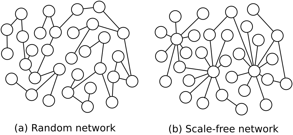
In the “scale-free” graphs edges are distributed not uniformly but with a high skew to some vertices. Such a vertices are often called “influencers”, vertices that are participating in a lot of edges. Like in typical social network most of people have from 10 to 100 followers but there are a few influencers that have millions of followers. If we compute the degree of each vertex as a count of its neighbors and plot the dependency between degree and the fraction of vertices with such a degree \( \mathbb{P}_k (k) \) we can see something like this:
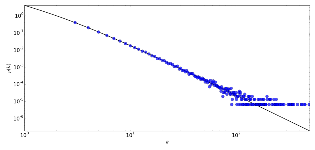
So, if we just split the adjacency list by vertices we will have a huge data skew in partitions. And we try to run any parallel version of algorithms on such a split, it will be far away from the perfect. Because, for example, the process that will process vertex with degree 10 will do 100,000 times less work than a process that is processing influencer with a million of neighbors.
And it is beside the fact that an implementation of the distributed lookup tables itself is not trivial.
“Two-phase” algorithm
The desire to distribute our graph and run parallel algorithms on top leads us to the map-reduce graph processing. Because we are talking about connected components problem, I would like to explain the algorithm from Kiveris, Raimondas, et al. “Connected components in MapReduce and beyond.” Proceedings of the ACM Symposium on Cloud Computing. 2014.. The algorithm if often named as “two-phase” or “big-star small-star” (by names of phases). While it is quite an old algorithm, I still see it as the best balance of performance and simplicity of the implementation.
Before we go to the algorithm itself, let me add a couple of words why Map-Reduce.
Why Map-Reduce?
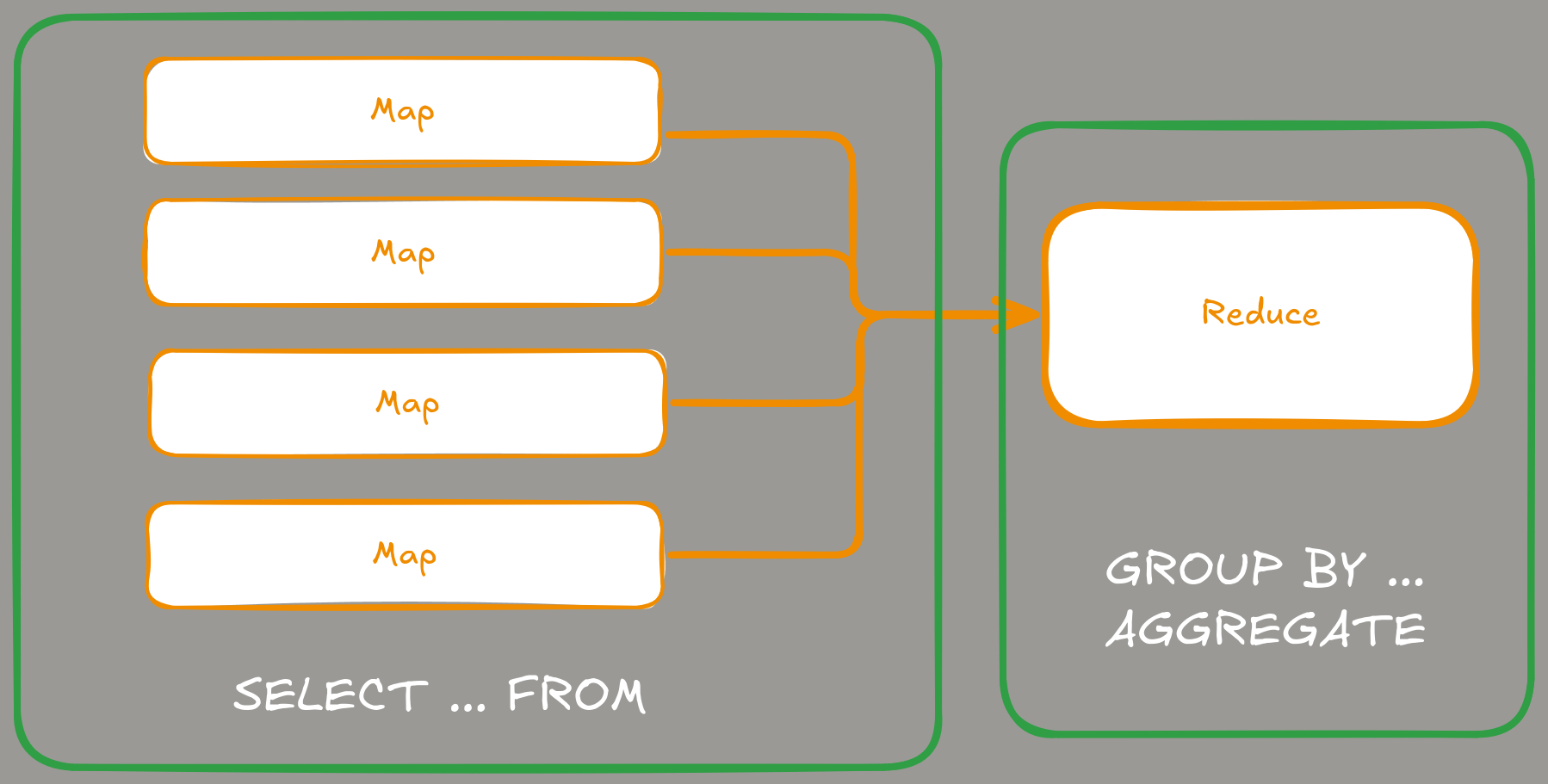
Although MapReduce is often associated with Hadoop or Apache Spark projects from years past, it is actually better than one might think. The cool thing about the MapReduce approach is that almost anything expressed in terms of the MR framework can easily be ported to operations on relations (SQL scripts, in other words). The Map-phase is just a SELECT ... FROM ... operation when we are processing each row in the atomic way. The Reduce-phase is GROUP BY + AGGREGATE operations (sometimes with a JOIN before it) when we are aggregating selected columns using an aggregation state.
Another good part of algorithms designed for MR framework is that they are written in a way of atomic operations and do not require any kind of the global state (with locks, syncs, and all the other fun). If you see “Algorithm XXX in Map-Reduce” in the name of the title of the scientific paper you can be almost sure that there won’t be anything like shared lookup hash table or the kind of global accumulator.
Finally, smart CS scientist developing MapReduce algorithms are aware of the skew curse as well as bottleneck in parallel algorithms, so most of papers specifically address worsen cases of loosing concurrency. Most of MR papers I read has a section about some additional tricks like how can we avoid skew and achieve an equal distribution of the data/compute across MR workers and reducers.
The idea of the two-phase algorithm explained
Hard math
Let’s begin with the definition of hard math from the paper itself.
We start with an undirected graph, \( G = (\{V\}, \{E\}) \). Note that the graph may actually be directed; in that case, the algorithm computes weakly connected components. In other words, edge directions are ignored entirely. This is sufficient for the aforementioned identity-resolution problem, as well as most strongly connected components algorithms are much more complex and less efficient.
Authors use the notation of \( \Gamma(u) = \{ w | (v, w) \in E \} \) for reference to the neighborhood of the vertex \( v \) and the notation \( \Gamma^{+}(v) \) for the so-called “extended” neighborhood: all the neighbors of \( v \) plus \( v \) itself.
We then attach labels \( \ell \) to each node. Labels should be “comparable”, for example, real numbers.
Next we are iteratively run two steps of MR, one is “small-star” and the second is “big-star”.
Small-star phase
Map \((u; v)\):
if \(\ell_v \leq \ell_u\) then
\(\quad\) Emit \((u; v)\).
else
\(\quad\) Emit \((v; u)\).
end if
Reduce \((u; N \subseteq \Gamma(u))\):
Let \(m = \arg\min_{v \in N \cup \{u\}} \ell_v\).
Emit \((v; m)\) for all \(v \in N\).
Big-star phase
Map \((u; v)\):
Emit \((u; v)\) and \((v; u)\).
Reduce \((u; \Gamma(u))\):
Let \(m = \arg\min_{v \in \Gamma^{+}(u)} \ell_v\).
Emit \((v; m)\) for all \(v\) where \(\ell_v > \ell_u\).
I’m not going to put here the proof of the convergence of the algorithm as well as the proof of the complexity. I would like to mention only that the overall complexity is \( O({\log}^2 n) \) of Map-Reduce iterations.
Intuition
Let’s take the small graph and see how these iterations work. I will use the small test graph from the Linked Data Benchmark Council (LDBC). The graph has the following edges:
| src | dst |
|---|---|
| 1 | 2 |
| 1 | 3 |
| 2 | 3 |
| 2 | 4 |
| 3 | 9 |
| 6 | 7 |
| 6 | 8 |

Preparation
Let’s use DuckDB and run map-reduce iterations of the algorithm as SQL operations in DuckDB.
sem@fedora:~$ duckdb
v1.0.0 1f98600c2c
Enter ".help" for usage hints.
Connected to a transient in-memory database.
Use ".open FILENAME" to reopen on a persistent database.
And create our edges table:
D CREATE TABLE edges AS SELECT * FROM
  (VALUES (1, 2), (1, 3), (2, 3), (2, 4), (3, 9), (6, 7), (6, 8))
  edges(src, dst);
First, we need to assign a real number to each vertex. However, since our vertices already have IDs, we can use those instead.
Large-star
Large-star phase actually means “connects all strictly larger neighbors to the min neighbor (including self)”. Before doing this we should also symmetrize the graph (Emit \((u; v)\) and \((v; u)\)) by duplicating edges with opposite direction. It is just like this in SQL.
(Symmetrized edges)
D SELECT DISTINCT src, dst FROM
  (SELECT src, dst FROM edges
  UNION (SELECT dst, src FROM edges));
┌───────┬───────┐
│  src  │  dst  │
│ int32 │ int32 │
├───────┼───────┤
│     3 │     9 │
│     1 │     3 │
│     6 │     7 │
│     7 │     6 │
│     8 │     6 │
│     2 │     4 │
│     2 │     1 │
│     3 │     1 │
│     1 │     2 │
│     4 │     2 │
│     6 │     8 │
│     9 │     3 │
│     3 │     2 │
│     2 │     3 │
├───────┴───────┤
│    14 rows    │
└───────────────┘
Minimal-neighbors including self (after symmetrization):
D CREATE TABLE min_nbrs AS SELECT src, LEAST(src, min_nbr) AS min_nbr FROM
  (SELECT src, MIN(dst) AS min_nbr FROM
  (SELECT DISTINCT src, dst FROM
    (SELECT src, dst FROM edges
    UNION (SELECT dst, src FROM edges))) GROUP BY src);
D SELECT * FROM min_nbrs;
┌───────┬─────────┐
│  src  │ min_nbr │
│ int32 │  int64  │
├───────┼─────────┤
│     1 │       1 │
│     2 │       1 │
│     3 │       1 │
│     4 │       2 │
│     6 │       6 │
│     7 │       6 │
│     8 │       6 │
│     9 │       3 │
└───────┴─────────┘
To check the convergence we compute the total sum of minimal neighbors and if this value did not decrease after one iteration it means that algorithm converged. SELECT sum(min_nbr) FROM min_nbrs with a result 25:
D SELECT SUM(min_nbr) FROM min_nbrs;
┌──────────────┐
│ sum(min_nbr) │
│    int128    │
├──────────────┤
│           26 │
└──────────────┘
Now we need to connect all neighbors to minimal neighbor: \((v; m)\) for all \(v \in N\)
D CREATE TABLE edges1 AS SELECT DISTINCT e.dst AS src, n.min_nbr AS dst FROM edges AS e JOIN min_nbrs AS n ON e.src = n.src;
D SELECT * FROM edges1;
┌───────┬───────┐
│  src  │  dst  │
│ int32 │ int64 │
├───────┼───────┤
│     2 │     1 │
│     3 │     1 │
│     4 │     1 │
│     7 │     6 │
│     8 │     6 │
│     9 │     1 │
└───────┴───────┘
Small-star
For the small-star, we need to compute minimal neighbors but this time without symmetrization. The result is the following:
D CREATE TABLE min_nbrs1 AS SELECT src, MIN(dst) as min_nbr FROM edges1 GROUP BY src;
D SELECT * FROM min_nbrs1;
┌───────┬─────────┐
│  src  │ min_nbr │
│ int32 │  int64  │
├───────┼─────────┤
│     2 │       1 │
│     3 │       1 │
│     4 │       1 │
│     7 │       6 │
│     8 │       6 │
│     9 │       1 │
└───────┴─────────┘
And we need to connect all smaller neighbors to the minimal neighbor:
D CREATE TABLE edges2 AS
  SELECT DISTINCT src, dst FROM
  (SELECT m.min_nbr AS src, e.dst FROM edges1 AS e JOIN min_nbrs1 AS m on e.src = m.src
  UNION (SELECT min_nbr AS src, src AS dst FROM min_nbrs1));
D SELECT * FROM edges2;
┌───────┬───────┐
│  src  │  dst  │
│ int64 │ int64 │
├───────┼───────┤
│     1 │     3 │
│     6 │     7 │
│     1 │     4 │
│     1 │     9 │
│     6 │     6 │
│     1 │     2 │
│     1 │     1 │
│     6 │     8 │
└───────┴───────┘
Actually the algorithm have converged already. To get the result we just need to select src from this “edges”. We need all the vertices as a table:
D CREATE TABLE vertices AS
  SELECT DISTINCT src AS id FROM
  (SELECT src FROM edges UNION
  (SELECT dst FROM edges));
  D SELECT * FROM vertices ORDER BY id;
  ┌───────┐
  │  id   │
  │ int32 │
  ├───────┤
  │     1 │
  │     2 │
  │     3 │
  │     4 │
  │     6 │
  │     7 │
  │     8 │
  │     9 │
  └───────|
And do a join:
D SELECT v.id, COALESCE(e.src, v.id) AS comp FROM
  vertices AS v LEFT JOIN edges2 AS e
  ON v.id = e.dst
  ORDER BY v.id;
┌───────┬───────┐
│  id   │ comp  │
│ int32 │ int64 │
├───────┼───────┤
│     1 │     1 │
│     2 │     1 │
│     3 │     1 │
│     4 │     1 │
│     6 │     6 │
│     7 │     6 │
│     8 │     6 │
│     9 │     1 │
└───────┴───────┘
And the result is correct :)

Balance of performance, simplicity, and flexibility
The paper I mentioned is quite old, from 2014 and there have been some recent works on connected components in MapReduce/SQL. However, I still consider the “Two-Phase” algorithm to be the best compromise between performance and ease of understanding and implementation. The algorithm is so simple that it can be implemented using only the built-in features of most DataFrame libraries and SQL engines. Additionally, the algorithm is perfectly suited for a distributed approach. It requires only one table, edges, and does not require any global state. The amount of communication across the cluster is also relatively small.
This algorithm is implemented in GraphFrames, where I am currently the most active maintainer. Because of that, when I started experimenting with Apache DataFusion for graph processing, I choose “Two-Phase” as a basis.
Implementation in Apache DataFusion
Now it’s time of the most interested part: an implementation of the algorithm above in Apache DataFusion and Rust.
About Apache DataFusion
Apache DataFusion is an extensible query engine written in Rust that provides high-performance execution of SQL and DataFrame operations. Its modular design allows developers to embed, extend, and customize its functionality for various data processing tasks. Focused on performance and safety, DataFusion leverages Rust’s zero-cost abstractions and memory safety guarantees. DataFusion supports reading and writing data in multiple formats, such as Parquet, CSV, and JSON. It also enables the optimization and execution of relational and analytical workloads. Although it is traditionally used for traditional data processing, its flexible architecture opens doors to more specialized applications, such as processing graph algorithms, making it an interesting candidate for unconventional use cases.
Implementation
Structures and constants
We will define a graph as two DataFusion DataFrame objects:
#[derive(Debug, Clone)]
pub struct GraphFrame {
    pub vertices: DataFrame,
    pub edges: DataFrame,
}
It is the same approach used in the GraphFrames project, which is quite flexible because it allows you to store not only the graph itself, but also its attributes. It’s similar to a labeled property graph model.
When we have a graph struct, we can define a Connected Components implementation. It is nice to return from the algorithm not only a DataFrame with mapping from ID to a component, but also an amount of iterations and the convergence parameter.
#[derive(Debug, Clone)]
pub struct ConnectedComponentsOutput {
    pub data: DataFrame,
    pub num_iterations: usize,
    pub min_nbr_sum: Vec<i128>,
}
We should also define a couple of constants.
pub const COMPONENT_COL: &str = "component";
const MIN_NBR: &str = "min_nbr";

/// (constants from the GraphFrame definition)
/// Column names for the vertex id column.
pub const VERTEX_ID: &str = "id";
/// Column names for the edge source column.
pub const EDGE_SRC: &str = "src";
/// Column names for the edge destination column.
pub const EDGE_DST: &str = "dst";
Utilities
Iterations of two-phase algorithm contains computing minimal neighbors in both symmetrized and plain graph. It would be better to define a function for it to avoid code duplication.
fn min_neighbours(edges: &DataFrame, symmetrize: bool) -> Result<DataFrame> {
    // symmetrize edges if needed
    let ee = if symmetrize {
        edges.clone().union(edges.clone().select(vec![
            col(EDGE_DST).alias(EDGE_SRC),
            col(EDGE_SRC).alias(EDGE_DST),
        ])?)?
    } else {
        edges.clone()
    };
    ee.aggregate(
        vec![col(EDGE_SRC).alias(VERTEX_ID)],
        vec![min(col(EDGE_DST)).alias(MIN_NBR)],
    )?
    .select(vec![
        col(VERTEX_ID),
        when(col(VERTEX_ID).lt(col(MIN_NBR)), col(VERTEX_ID))
            .otherwise(col(MIN_NBR))?
            .alias(MIN_NBR),
    ])
}
We need also a way to estimate the convergence. It will be simpler to do it as a function as well. To avoid an overflow when doing sum over Long IDs it is better to convert to Decimal128 first.
async fn min_nbr_sum(min_neighbours: &DataFrame) -> Result<i128> {
    min_neighbours
        .clone()
        .aggregate(
            vec![],
            vec![sum(cast(col(MIN_NBR), DataType::Decimal128(38, 0))).alias(MIN_NBR)],
        )?
        .collect()
        .await?
        .first()
        .ok_or(datafusion::error::DataFusionError::Internal(
            "failed to calculate and collect min_nbr_sum: result is empty".to_string(),
        ))?
        .column(0)
        .as_any()
        .downcast_ref::<Decimal128Array>()
        .ok_or(datafusion::error::DataFusionError::Internal(
            "failed to get min_nbr_sum as Decimal128Array".to_string(),
        ))
        .map(|a| a.value(0))
}
Preparations
We need to prepare our graph first. It is a trick from the original paper, that to improve the convergence we can re-order edges first, so the src < dst.
// Preparation of the graph:
// - removing self-loops
// - changing edge direction so SRC < DST
// - de-duplicate edges
let vertices = self.graph_frame.vertices.clone();
let original_edges = self.graph_frame.edges.clone();

let no_loops_edges = original_edges.filter(col(EDGE_SRC).not_eq(col(EDGE_DST)))?;
let ordered_by_direction_edges = no_loops_edges.select(vec![
    when(col(EDGE_SRC).lt(col(EDGE_DST)), col(EDGE_SRC))
        .otherwise(col(EDGE_DST))?
        .alias(EDGE_SRC),
    when(col(EDGE_SRC).lt(col(EDGE_DST)), col(EDGE_DST))
        .otherwise(col(EDGE_SRC))?
        .alias(EDGE_DST),
])?;
let deduped_edges = ordered_by_direction_edges.distinct()?;
And we need some mutable variables to store iteration, iteration metrics and the current neighbors sum.
let mut iteration = 0usize;
let mut metrics = Vec::<i128>::new();
let mut converged = false;
On each iteration we need to have minimal neighbors of the current edges as well we will change edges during iterations. Let’s do some preparations.
let mut minimal_neighbours_1 = min_neighbours(&deduped_edges.clone(), true)?;
let mut last_iter_nbr_sum = min_nbr_sum(&minimal_neighbours_1.clone()).await?;
metrics.push(last_iter_nbr_sum);
let mut current_edges = deduped_edges.clone().cache().await?;
Iterations
Everything is ready and we can finally write an iterative process.
while !converged {
iteration += 1;
// large-star step:
// connects all strictly larger neighbors to the min neighbor (including self)
current_edges = current_edges
.join_on(
minimal_neighbours_1.clone(),
JoinType::Inner,
vec![col(EDGE_SRC).eq(col(VERTEX_ID))],
)?
.select(vec![
col(EDGE_DST).alias(EDGE_SRC),
col(MIN_NBR).alias(EDGE_DST),
])?
.distinct()?
.cache()
.await?;
// small-star step:
// computes min neighbors (excluding self-min)
let minimal_neighbours_2 = min_neighbours(¤t_edges.clone(), false)?
.cache()
.await?;
// connect all smaller neighbors to the min neighbor
current_edges = current_edges
.clone()
.join_on(
minimal_neighbours_2.clone(),
JoinType::Inner,
vec![col(EDGE_SRC).eq(col(VERTEX_ID))],
)?
.select(vec![col(MIN_NBR).alias(EDGE_SRC), col(EDGE_DST)])?
.filter(col(EDGE_SRC).not_eq(col(EDGE_DST)))?
.union(minimal_neighbours_2.select(vec![
col(MIN_NBR).alias(EDGE_SRC),
col(VERTEX_ID).alias(EDGE_DST),
])?)?
.distinct()?
.cache()
.await?;
minimal_neighbours_1 = min_neighbours(¤t_edges.clone(), true)?
.cache()
.await?;
let current_sum = min_nbr_sum(&minimal_neighbours_1.clone()).await?;
if current_sum == last_iter_nbr_sum {
converged = true;
} else {
last_iter_nbr_sum = current_sum;
metrics.push(current_sum);
}
}
Post-processing
The last thing we should do is to connect vertices and components and wrap everything to return.
Ok(ConnectedComponentsOutput {
    data: vertices
        .join_on(
            current_edges,
            JoinType::Left,
            vec![col(VERTEX_ID).eq(col(EDGE_DST))],
        )?
        .select(vec![
            col(VERTEX_ID),
            when(col(EDGE_SRC).is_null(), col(VERTEX_ID))
                .otherwise(col(EDGE_SRC))?
                .alias(COMPONENT_COL),
        ])?,
    num_iterations: iteration,
    min_nbr_sum: metrics,
})
Benchmarking
I used graph from LDBC to benchmark my solution. I was running benchmarks on my ThinkPad Laptop that has 38 GB of RAM and i5-1335U CPU (12 cores). Something was working on background, like text editor, music player and browser, so benchmarks are not perfect. But I still want to share the numbers to understand the scale.
| Property | Value |
|---|---|
| Num vertices | 4,610,222 |
| Num edges | 129,333,677 |
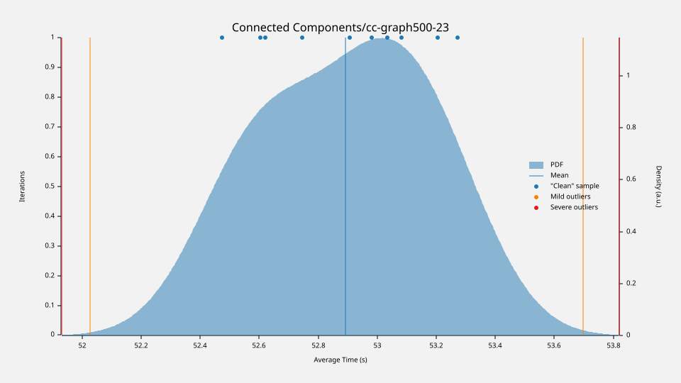
The average running time is about 53 seconds (not including I/O). That’s not bad at all; it’s on the same level as the BFS-based implementation from NetworkX (which takes ~47 seconds without I/O). The good news is that I/O is fast, thanks to the highly optimized CSV reader from DataFusion. It’s around 20 times faster than NetworkX. Additionally, memory consumption is half that of NetworkX (thanks to arrow-rs, which powers the DataFusion DataFrame).
Performance compared to Spark GraphFrames
My DataFusion-based implementation is around 4-5 times faster than Spark-based GraphFrames on the same LDBC graph when the data fits into the memory. When the data no longer fits into memory… Well, DataFusion crashes, while GraphFrames only slows down by spilling. I will explain the reason in the next section. Long story short, DataFusion does not support persistence (i.e., caching) to disk or memory+disk, whereas Spark does. In case you were wondering, iterative algorithms in DataFusion won’t work without caching. The optimizer is cool, but unfortunately, it cannot perform miracles.
Source code
The code I mentioned above is a part of my graphframes-rs project I’m working on in my free time. While there is no purpose of the project (I will explain further why), it is still funny. And of course you can star the project if you like it (or this post). Stars in GitHub is the best reward :)
DataFusion by eyes of Spark developer
We have finished discussing the main topic of this post. Now, I would like to share my first impressions of Apache DataFusion. I would describe myself as an experienced Apache Spark user. I’m not an expert who contributes to the project itself, but I maintain a few libraries built on top of it. I will mostly compare my impression of DataFusion with my impression of Spark. My impressions are not those of a user, but rather those of a library developer. If you are not a DataFusion expert but want to build something on top of it, my perspective may be useful.
Good
Let’s start from the good.
Performance
It’s excellent! Really excellent! It’s four to five times faster than Spark. Memory consumption is slightly lower, and I/O is faster. Another cool feature of DataFusion is that you can write UDFs that are as fast as native expressions. In Apache Spark, you can also write UDFs, but they fall back to the Volcano iterator mode with a huge memory overhead, no JIT, and a huge garbage collector load. Of course, there’s an option to write a Catalyst native expression in Spark, but I’d say, “May the Force be with you,” to anyone who wants to try it. It’s possible, but it’s mind-blowing. There are no clear docs (only old blog posts), no clear way to debug, and no IDE support. You have to write Java code as strings because that’s how the code generation works.
DataFusion is different. You can just express you logic in arrow-rs, wrap to ScalarUDF and it works in exactly the same way like all the native functions. That are benefits of columnar model!
Developer experience
It is nice! Best support in all the IDEs with rust analyzer opposite to the Scala world when you have only metals LSP that does not support mixed Java-Scala projects at all and IntelliJ IDEA. As an ASF committer I have IDEA Pro for free (huge thanks to JetBrains), but even IDEA is very buggy for Scala… Like IDEA does not respect SBT configurations so, for example, for tests and debugging you have only CLI, etc.
Cargo and rust analyzer are providing, imo, much better experience compared to SBT.
Bad
Let’s now go to bad parts. I will try to explain all my pain from some unobvious things and hours of googling and debugging. Before we go, I should explicitly mention that I’m not trying to say that DataFusion is bad. I just want to say that it may be hard. Hard even compared to Spark (that is far away from project that are simple to work with). It is my personal experience by the end.
NOTE: It is actually possible that I’m just using DataFusion in a wrong way or missed something in documentation. And problems I will mention are not problems at all.
Debugging
If one works one day with Spark based projects they should now how painful debugging may be. Everything is lazy, code is generated and compiled at runtime, a long chain of abstractions… I was really hoping that in DataFusion I will just but some breakpoints, click “debug” and will be happy. Of course not. Everything is async / tokio, everything is lazy. Behind that is arrow-rs that is not actual “data” but some cryptic combination of buffers, offsets and nulls. I made a couple of attempts but failed and ended by old-school collect + print way. Not worsen than Spark by the end :)
Error messages
Everyone “loves” Spark error messages. In the JVM world there is a meme, that developers should have two monitors. One horizontal for class names and the second a vertical one for stacktraces.

I was really expecting something better from DataFusion… While it is different from Spark in some ways, it is still quite strange. Like you get an error Wrong Plan. Really, that’s it, only this message. No row, no class name, nothing. Just “your plan is wrong, good luck with finding why”. Or, for example, Error: Plan("Field id not found in struct"). What field? What struct? At least, from where did come? No, only hard-mode, unfortunately… What about datafusion Unnest should be rewritten to LogicalPlan::Unnest before type coercion? Really, does anyone understand what does it mean? At least there is a reference to unnest and it reduce the scope of investigation :)
Or what do you think about the fact that you just cannot use CASE-WHEN inside MAP? It is not documented anywhere (at least I did not find), but you just cant. It fails with some cryptic error about bad plan…
MapType is a very interesting thing in DataFusion. For example, did you know that the implementations of MapType in arrow-rs and DataFusion have a funny difference that you’ll notice after a couple of hours of digging if you decide to write the UDF? The underlying arrow-rs names the keys and values fields “keys” and “values,” respectively, but the corresponding DataFusion wrapper names them “key” and “value.” Live with it.
Apache Spark at least tells you from where the error is coming (of course only if your monitor is big enough to show you 5000 lines of stacktrace)…
NOTE: After my work with DataFusion I have a very strong feeling that all the projects around DataFusion are done by engineers, who are contributors of the DataFusion itself. While it is not bad at all and I’m definitely not the person who have a right to blame anyone, I should mention that fact. In the ecosystem around Spark it is very different and most of the projects are done by independent contributors.
Rust may be annoying
Most probably I just do not know how to write in Rust in the right way. But as a side person who is not very familiar with language I would say, that compiler can be really annoying. And the only real way to fight Rust for me was to add endless clone everywhere. I don’t think that cloning the lazy DataFrame (in other words, a LogicalPlan) is expensive, but it looks really strange. Like self.graph.vertices.clone(), column.init_expr.clone(), message.expr.clone(), and so fourth and so on.

Principal limitations
At the end I would like to mention what I think are some principal limitations of DataFusion for graph algorithms.
Not distributed (yet)
It is not distributed. While it is not a problem of the project itself, it makes senseless to write any Map-Reduce like algorithm with it. The golden rule of graph processing is if your graph fits into the memory process it with a single-node algorithms. Yes, DataFusion may provides some benefits like a lot of ready to use connectors, zero-copy transfer from tables to graphs and very low memory consumption. But Map-Reduce algorithms are not optimal and slower compared to classical graph routines. It is an obvious fact, simply because MR-algorithms are designed for distributed processing.
No off-memory persistence
That is the bigger limitation because it affects not only graphs but also most iterative algorithms. Although DataFusion can spill data to disk and work in out-of-core mode (meaning it can process more data than your RAM), there is no way to persist intermediate results to disk or memory plus disk.
Apache Spark provides persist method with configurable StorageLevel), but DataFusion provides only cache that persist the data to memory. And even if the engine itself can handle out-of-core problems, you cannot write iterative algorithms for out-of-core problems because you cannot store intermediate results :(
Conclusion
I still don’t see what may be the place for the DataFusion in Graphs landscape. Like yes, you can write graph algorithms but without an ability of distributed processing or, at least, out-of-core processing, it does not make real sense. If the graph fits into the memory and you can process it in memory it will be much better to use NetworkX (or IGraph, or graph-tools, or RewtworkX, or any other pure graph library). I hope to see DataFusion distributed one day or maybe to see better APIs for out-of-core problems (especially persisting options). But if you like the post, please star the repo, it is the best reward for me :)
https://github.com/SemyonSinchenko/graphframes-rs/tree/main
I hope it was interesting. And I would like to mention it again: I’m not trying to blame anyone or criticize DataFusion as a project. It is beautiful, perfect piece of software. It is maintained by really cool engineers, rock stars! I just wanted to share my small impression, like what may the mediocre developer feel working with DataFusion.