FastRP graph embeddings with Apache DataFusion

TLDR;

FastRP is an algorithm for learning graph vertex representations (embeddings). This is a hot topic today because embeddings have many applications: from nearest neighbors search to agentic retrieval, GraphRAG and Graph Machine Learning. The algorithm is fast, easy to implement, intuitive and efficient. In this post I will explain the idea and show how to implement it in a fully out-of-core mode using Apache DataFusion and Rust.

Introduction

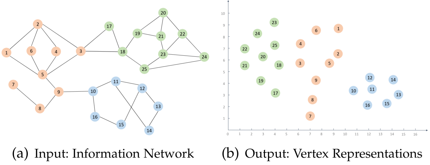
Vertex Representation Learning

I already made a deep dive about Vertex Representation Learning and usage of node embeddings.

Why not Node2Vec?

While the Node2Vec (Grover, Aditya, and Jure Leskovec. "node2vec: Scalable feature learning for networks." Proceedings of the 22nd ACM SIGKDD international conference on Knowledge discovery and data mining. 2016.) algorithm became the de-facto standard of the industry for vertex representation learning, there are some problems with. At first, generation of random walks may be an expensive and long process. Typical default values for most implementations are L=80 for walks length and N=10 to number of parallel chains. That means we need to make \( O(|V| \cdot L \cdot N) \) operations of choosing the next node and this one is hard to accelerate via things like SIMD. The second problem is the amount of data generated by random walks. For the graph500-24 graph with 8 million of nodes, this means we need to process somehow approximately 50 GB of uint64 values (assuming long IDs, because we are talking here about big graphs and barely want to limit ourselves by 2B nodes cap). And the last and, probably, the biggest problem is that the Word2Vec itself is a bad choice for graph problems. While the connection between the words coocurrence in sentences and nodes in random walks is clear, Word2Vec was designed for natural Language Processing (NLP). Practical NLP systems often cap their vocabulary at the most frequent \(10^5\)–\(10^6\) tokens, whereas graph embedding systems may need to represent every node in a graph with tens or hundreds of millions of nodes (the so-called extreme scale embeddings problem).

FastRP

Chen, Haochen, et al. "Fast and accurate network embeddings via very sparse random projection." Proceedings of the 28th ACM international conference on information and knowledge management. 2019.

The algorithm itself is very intuitive. We start from very sparse random embeddings on each node. On each iteration we are aggregating all the embeddings from node's neighbors and compute a new node's embedding as sum or avg.

A bit more about FastRP

I gave an oversimplified explanation while the reality is slightly more tricky. FastRP does not just aggregation, but normalize the embeddings: each neighbor's embedding is divided by the neighbor's output degree (\( L_1 \)) or squar root of the output degree (\( L_2 \)). As well, the final embedding is a weighted sum of embeddings from iterations with typical weights like [0.0, 1.0, 1.0, 1.0] (the random initialization does not contribute to the output). For more details I will add also a reference to the paper.

Let's illustrate how it works on a simple example: Zachary Karate Club Network.

We can use \( d=2 \) as a dimension, so initially each node of the graph is represented by two random numbers. Then we will do 5 iterations of the algorithm.

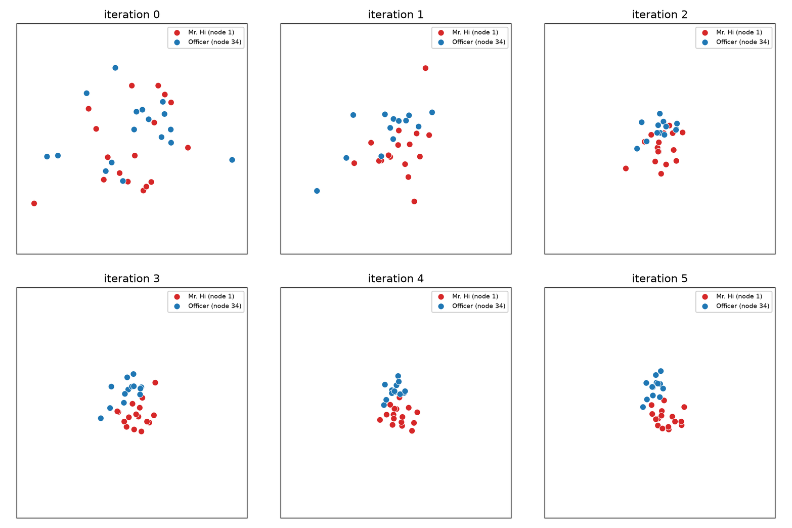
Illustration of FastRP work — FastRP over Zachary Karate Club network, 5 iterations. Colors are ground truth communities. Coordinates are 1st and 2d values of FastRP embedding

As one may see, on the first iteration all the nodes are randomly distributed in the embedding space (\( \mathbb{R}^2 \)). After a few iterations, nodes form the dense bubbles around the known ground truth communities. And the two factions become visually more separable.

NOTE: Linear separability of nodes is not the only goal of the node representation learning as well not the best quality metric. But it is the best for explanation of how things work. Please, refer to the paper for more tetails how were they estimating the FastRP embeddings quality.

FastRP in terms of operations on relations

Let's imagine we made three SQL User Defined Functions:

fastrp_init(id, dim, seed): uses id, an expected dimension dim and a global random seed seed as input; generates extremely sparse embeddings or list<float> with the size dim of values [-1.0, 0.0, 1.0]; we are choosing the \( \pm 1 \) with a probability \( \rho = \frac{1.0}{2 \sqrt{q} } \) where \( q \) is the largest power of two that does not exceed the dim.
vector_sum(vectors): an aggregation function that takes multiple list<float> of the same size and return an element-wise sum.
vector_div_by_scalar(vector, value): takes a list<float> and a scalar value, divide each elemen of the list by it.

Then we can express the FastRP algorithm as a series of SQL operations. Let's say we have edges and vertices tables. The initial value of fastrp embeddings are:

  CREATE TABLE embeddings_0 AS
  SELECT id, out_deg, fastrp_init(id, 128, 42) AS embedding;

Iterations can be expressed in the following way:

  CREATE TABLE embeddings_1 AS SELECT dst AS id, vector_sum(embedding) AS embedding
  FROM (
    SELECT src, dst, vector_div_by_scalar(embedding, out_deg) FROM
    edges
    LEFT JOIN embeddings_0
    ON src = id
  ) GROUP BY dst;

Long story short. At each iteration we left join the current embeddings state to edges and get triplets: src, dst, src_embedding – a table that contains all the edges of the graph (src, dst) and an embedding of the source node. We divide the embedding by the out degree of this node and aggregate all the embeddings using sum and grouping by the destination node. In simple words it means that \( v_{k+1}^j \) embedding is just a sum of \( v_k \) embeddings of all the \( j-th \) neighbors: \( v_{k + 1}^j = \sum_{i \in N_j} v_k^i \).

In Apache DataFusion it is just a simple loop:

  let message = match self.normalization {
    FastRPNormalization::None => col(EMBEDDING),
    FastRPNormalization::L1 => vec_scale_expr(
      col(EMBEDDING),
      lit(1.0f64) / cast(col(DEGREE), DataType::Float64),
    ),
    FastRPNormalization::L2 => vec_scale_expr(
      col(EMBEDDING),
      lit(1.0f64) / sqrt().call(vec![cast(col(DEGREE), DataType::Float64)]),
    ),
  };
  // .... //
  for t in 1..=self.iterations {
    let triplets = edges.clone().join_on(
      state.clone(),
      JoinType::Inner,
      vec![col(EDGE_SRC).eq(col(VERTEX_ID))],
    )?;
    let messages = triplets.select(vec![
      col(EDGE_DST).alias(VERTEX_ID),
      message.clone().alias(EMBEDDING),
    ])?;
    let aggregated = messages.aggregate(
      vec![col(VERTEX_ID)],
      vec![vec_sum_expr(col(EMBEDDING), self.dim).alias(EMBEDDING)],
    )?;
    state = states_checkpointer
      .push_pre_sorted(&ctx, &format!("state-{t}"), aggregated, VERTEX_ID)
      .await?;
      states.push(state.clone());
  }

Experiments

Visual Representation

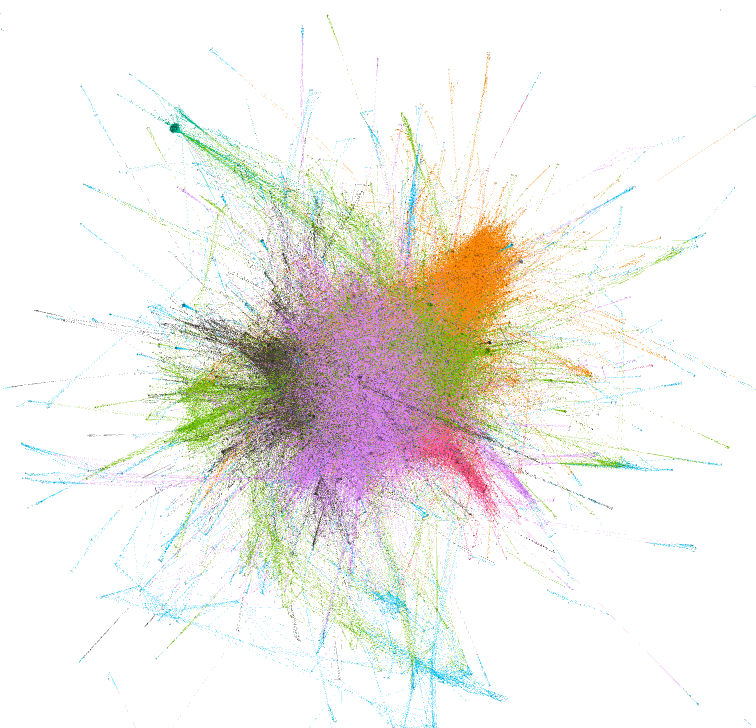
The first "quality" test for the embeddings is "visual". I took the Enron Emails Dataset, a communication network with 37k nodes and 184k edges. I made embeddings for the netowrk and used as an input for the KMeans clustering algorithm I implemented recently using DataFusion and Rust.

KMeans clustering with k=8 over FastRP embeddings of the Enron-emails graph

From my subjective point of view, this is quite a good clustering. Embeddings are separating well 4 central clusters as well all the periphery nodes are combined into a separate K-Means cluster.

Machine Learning Test

The second "quality" test is to try to fit machine learning models on FastRP embeddings to see how well are they encoding information about graph nodes.

I run three small node-classification problems from the Karate Club Datasets. Results are somewhat I expected to see: FastRP embeddings predictive power is on par with Node2Vec embeddings while the wall time is 500-600 times better. This matches the results got by the FastRP authors.

Dataset	Nodes	Edges	Node2Vec AUC	Node2Vec Wall, s	FastRP AUC	FastRP Wall, s
wikipedia	11,631	182,404	0.8534	2,036	0.8225	3
github	37,700	289,003	0,8735	6,411	0.834	12
twitch	7,126	35,324	0.5847	503	0.5854	1

NOTE: This is not the fastest possible implementation of the Node2Vec. I used one from the Karate Club Project which is based on NetworkX for random walks generation and gensim.models for Word2Vec implementation. Meanwhile my numbers are matching overall the FastRP paper: authors saw the similar order of magnitude difference in the wall time with very close numbers in output quality.

Performance

I made a test run on graph500-24 from the LDBC Collection. The end2end run, from FastRP embeddings to KMeans clustering was around 15 minutes using 24 GB RAM pool and 4 CPU-cores. Not the blazingly fast, but quite a scalable.

A screenshot of the algorithm run on graph500-24

Of course, this JOIN - GROUP BY - AGGREGATE based implementation is fully out of core. At any moment of time the maximal amount of data that needs to be materialized is proportional to the batch size and number of DataFusion workers (\( \simeq O(BdW) \), \(B\) is a DataFusion batch size, \(d\) is an embedding dimension, \(W\) is number of Tokio workers), not the total amount of data. Since the edge stream and the embedding state are processed using streaming sort-merge joins and checkpointed between iterations, the implementation does not keep the graph or the full embedding state in RAM. For a fixed batch size, embedding dimension, and number of workers, the peak working memory is independent of \(|V|\) and \(|E|\). Larger graphs increase disk I/O and execution time, but not the RAM requirement.