Leveraging Time-Based Feature Stores for Efficient Data Science Workflows
In our previous post, we briefly touched upon the concept of ML feature stores and their significance in streamlining machine learning workflows. Today, we’ll again explore a specific type of feature store known as a time-based feature store, which plays a crucial role in handling temporal data and enabling efficient feature retrieval for data science tasks. In this post we’ll how a feature-lookup problem may be effectively solved in PySpark using domain knowledge and understanding how Apache Spark works with partitions and columnar data formats.
Precomputed features stored can significantly speed up the Data Science development process and simplify maintenance, lineage, and data quality tracking. By having a centralized repository of precomputed features, data scientists can easily access and reuse these features across multiple projects, eliminating the need to repeatedly compute them from scratch. This approach saves valuable time and computational resources, allowing data scientists to focus on model development and experimentation rather than feature engineering. Moreover, a feature store acts as a single source of truth for all features, ensuring consistency and reducing the risk of mismatch between different models or projects. It also simplifies lineage tracking, as the origin and transformations of each feature are well-documented and easily traceable. Additionally, data quality issues can be identified and addressed at the feature level, ensuring that all models consuming those features benefit from the improvements. By centralizing feature management, organizations can avoid the need to implement feature computation, lineage, and data quality tracking for each model separately, leading to a more efficient and maintainable Data Science workflow.
Understanding Time-Based Feature Stores
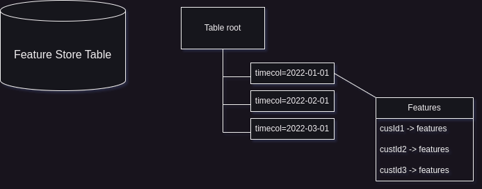
A time-based feature store is essentially a table that contains precomputed features for each customer at various timepoints over a recent period. This table is typically partitioned by a timecol column, which represents the date on which the features are up-to-date. Each partition within the table includes data in the form of a customer ID (custid) mapped to a set of features.
For example, consider a scenario where we have a feature store table with one thousand features computed for each customer ID and corresponding date (represented by the timecol partition column). The table structure would look something like this:
timecol (partition column) | custid | feature_1 | feature_2 | ... | feature_1000
Typical Use Case: Leveraging Feature Stores for Data Science Tasks
A common use case for leveraging a feature store arises when a data scientist has data in the form of customer_id -> (observation_date, observation, *additional_columns). The observation_date represents the date wheni, for example, a marketing communication was sent to a customer, and the observation represents the customer’s reaction to the marketing communication, such as whether the customer accepted the offer within a week after the communication or not. In terms of ML Models observation is like y variable.
The task at hand is to create a predictive machine learning model that can estimate the probability of success of a marketing communication for a given customer. To accomplish this, we need to create a dataset in the form of customer_id -> (observation_date, observation, *additional_columns, features), where the features are retrieved from the feature store.
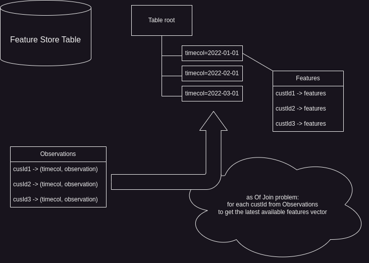
It is crucial to avoid leakage of features from the future and ensure that only the latest available features before the observation_date are used. This requirement leads to the “asOfJoin” problem, which involves joining the customer data with the feature store table based on the customer ID and the observation date.
The asOfJoin Problem
The asOfJoin problem revolves around finding the most recent set of features for each customer that were computed before a given observation date. It requires joining the customer data with the feature store table while considering the temporal aspect of the data.
Conceptually, the asOfJoin operation can be described as follows:
For each customer ID in the customer data:
    Find the latest available features in the feature store table
    where the timecol is less than or equal to the observation date
The asOfJoin problem is a common challenge in data science workflows, particularly when dealing with time-series data or scenarios where features need to be retrieved based on specific timepoints. In the upcoming sections, we’ll dive deeper into the asOfJoin problem, explore various approaches to solve it efficiently, and discuss how important for an engineer do not use generic algorithms blindly but put a domain knowledge into the solution code instead.
Data Generation and test setup
To simulate the described above workflow and asOfJoin let’s create few feature tables of different size and an observation table.
Data Generation Code
from uuid import uuid1

from datetime import datetime, timedelta
from random import random, randint
from pyspark.sql import SparkSession, functions as F, types as T, DataFrame, Row


spark = SparkSession.builder.master("local[*]").getOrCreate()

def generate_fs_schema(n: int) -> T.StructType:
    fields = [T.StructField("custid", T.StringType())]
    for i in range(n):
        fields.append(T.StructField(f"feature_col_{i}", T.DoubleType()))

    return T.StructType(fields=fields)

OBSERVATIONS_SCHEMA = T.StructType(
    [
        T.StructField("custid", T.StringType()),
        T.StructField("timecol", T.StringType()),
        T.StructField("observation", T.IntegerType()),
        T.StructField("additionalColA", T.StringType()),
        T.StructField("additionalColB", T.StringType()),
        T.StructField("additionalColC", T.StringType()),
        T.StructField("additionalColD", T.StringType()),
        T.StructField("additionalColE", T.StringType()),
        T.StructField("additionalColF", T.StringType()),
        T.StructField("additionalColG", T.StringType()),
        T.StructField("additionalColH", T.StringType()),
        T.StructField("additionalColI", T.StringType()),
    ]
)

N = 100_000

CUSTOMER_IDS_ALL = [uuid1() for _ in range(N)]

CUSTOMER_IDS_OBSERVATIONS = [uid for uid in CUSTOMER_IDS_ALL if random() <= .25]
DATES_ALL = [d.to_pydatetime() for d in pd.date_range(start="2022-01-01", end="2024-01-01", freq="ME")]


def generate_observations() -> DataFrame:
    rows = []
    for cid in CUSTOMER_IDS_OBSERVATIONS:
        rows.append(
            Row(
                custid=cid,
                timecol=datetime.strftime(DATES_ALL[randint(1, len(DATES_ALL) - 1)] - timedelta(days=randint(0, 20)), "%Y-%m-%d"),
                observation=randint(0, 1),
                additionalColA=random(),
                additionalColB=random(),
                additionalColC=random(),
                additionalColD=random(),
                additionalColE=random(),
                additionalColF=random(),
                additionalColG=random(),
                additionalColH=random(),
                additionalColI=random(),
            )
        )
    return spark.createDataFrame(rows, schema=OBSERVATIONS_SCHEMA)


def generate_fs_partition(schema: T.StructType, date_col: str) -> DataFrame:
    rows = []
    for cid in CUSTOMER_IDS_OBSERVATIONS:
        res = {}
        for col in schema.fields:
            if col.name == "custid":
                val = cid
            elif col.name == "observation":
                val = randint(0, 1)
            else:
                val = random()

            res[col.name] = val

        rows.append(Row(**res))

    return spark.createDataFrame(rows, schema)
The code starts by importing necessary libraries and creating a SparkSession.
- The
generate_fs_schemafunction is defined next, which takes an integernas input and generates aStructTypeschema for a feature store dataset; The schema includes a “custid” field of string type andnadditional fields named “feature_col_i” of double type; - The
OBSERVATIONS_SCHEMAis defined as aStructTyperepresenting the schema for an observations dataset (or train dataset in terms of ML workflow). It includes fields such as “custid”, “timecol”, “observation”, and additional columns from “additionalColA” to “additionalColI” that represents some additional features or informatin, for example a channel of merketing communication; - The code sets the value of
Nto 100,000, which represents the number of unique customer IDs to generate. TheCUSTOMER_IDS_ALLlist is created by generatingNunique customer IDs using theuuid1function. TheCUSTOMER_IDS_OBSERVATIONSlist is created by filtering theCUSTOMER_IDS_ALLlist based on a random probability of0.25; - The
DATES_ALLlist is created by generating a sequence of dates from “2022-01-01” to “2024-01-01” with a monthly frequency using thepd.date_rangefunction. For simplicity we will simulate the case when Feature Store Table has a monthly basis. In other words, we will have all the features for each customer once per month. - The
generate_observationsfunction is defined, which generates a DataFrame representing the observations dataset. It iterates over theCUSTOMER_IDS_OBSERVATIONSlist and creates a row for each customer ID with random values for the observation and additional columns. For avoiding a trivial case when observation dates match exactly to end of month we make also a random shift by 0-20 days back; - The
generate_fs_partitionfunction is defined, which generates a DataFrame representing a partition of the feature store dataset. It takes aStructTypeschema and a date column name as input. It iterates over theCUSTOMER_IDS_OBSERVATIONSlist and creates a row for each customer ID with random values for the feature columns.
The following code generates for us three observation datasets and three Feature Store tables of different size:
OBS = generate_observations()

OBS.write.mode("overwrite").parquet("data/OBSERVATIONS")
OBS.sample(0.5).write.mode("overwrite").parquet("data/OBSERVATIONS_SMALL")
OBS.sample(0.25).write.mode("overwrite").parquet("data/OBSERVATIONS_TINY")

SCHEMA_10 = generate_fs_schema(10)
SCHEMA_50 = generate_fs_schema(50)
SCHEMA_150 = generate_fs_schema(150)

for date in DATES_ALL:
    date_str = datetime.strftime(date, "%Y-%m-%d")
    generate_fs_partition(SCHEMA_10, date_str).write.mode("overwrite").parquet(f"data/FS_TABLE_10/timecol={date_str}")
    generate_fs_partition(SCHEMA_50, date_str).write.mode("overwrite").parquet(f"data/FS_TABLE_50/timecol={date_str}")
    generate_fs_partition(SCHEMA_150, date_str).write.mode("overwrite").parquet(f"data/FS_TABLE_150/timecol={date_str}")
Checking the generated data
We have three observation datasets:
- TINY:
1.1 Mb; - SMALL:
2.2 Mb; - REGULAR:
4.2 Mb;
And we have three feature store tables:
- 10 features:
65 Mb; - 50 features:
251 Mb; - 150 features:
717 Mb;
All three feature tables are partitioned by timecol:
> dust --depth 1 FS_TABLE_150/

  0B   ┌── _SUCCESS           │   0%
4.0K   ├── ._SUCCESS.crc      │   0%
 29M   ├── timecol=2022-01-31 │   4%
 29M   ├── timecol=2022-02-28 │   4%
 29M   ├── timecol=2022-03-31 │   4%
 29M   ├── timecol=2022-04-30 │   4%
 29M   ├── timecol=2022-05-31 │   4%
 29M   ├── timecol=2022-06-30 │   4%
 29M   ├── timecol=2022-07-31 │   4%
 29M   ├── timecol=2022-08-31 │   4%
 29M   ├── timecol=2022-09-30 │   4%
 29M   ├── timecol=2022-10-31 │   4%
 29M   ├── timecol=2022-11-30 │   4%
 29M   ├── timecol=2022-12-31 │   4%
 29M   ├── timecol=2023-01-31 │   4%
 29M   ├── timecol=2023-02-28 │   4%
 29M   ├── timecol=2023-03-31 │   4%
 29M   ├── timecol=2023-04-30 │   4%
 29M   ├── timecol=2023-05-31 │   4%
 29M   ├── timecol=2023-06-30 │   4%
 29M   ├── timecol=2023-07-31 │   4%
 29M   ├── timecol=2023-08-31 │   4%
 29M   ├── timecol=2023-09-30 │   4%
 29M   ├── timecol=2023-10-31 │   4%
 29M   ├── timecol=2023-11-30 │   4%
 29M   ├── timecol=2023-12-31 │   4%
717M ┌─┴ FS_TABLE_150
Why partitioning is important?
Apache Spark’s optimizer can leverage information about partitioning and min/max values from Parquet file headers to optimize query execution and reduce the amount of data that needs to be read.
Partitioning:
- When data is partitioned based on certain columns, Spark can use this information to prune partitions that are not relevant to the query.
- If a query has filters on the partitioning columns, Spark can identify which partitions satisfy the filter conditions and skip reading the irrelevant partitions entirely.
- This partition pruning optimization can significantly reduce the amount of data scanned and improve query performance.
Min/Max Values in Parquet File Headers:
- Parquet files contain metadata in their headers, including the minimum and maximum values for each column within the file.
- Spark’s optimizer can utilize this information to determine if a file needs to be read based on the query’s filter conditions.
- If the filter condition falls outside the range of min/max values for a column in a Parquet file, Spark can skip reading that file altogether.
- By avoiding unnecessary file scans, Spark can optimize query execution and reduce the amount of I/O operations.
Combining Partitioning and Min/Max Values:
- When data is partitioned and stored in Parquet format, Spark can leverage both partitioning information and min/max values for optimization.
- Spark can first prune irrelevant partitions based on the partitioning scheme and query filters.
- Within the remaining partitions, Spark can further utilize the min/max values from the Parquet file headers to determine which files need to be read.
- By combining these optimizations, Spark can significantly reduce the amount of data scanned and improve query performance.
NOTE: By leveraging partition pruning, projection pushdowm and predicate pushdown it is possible to allow Spark/PySpark to work in a hard out-of-core mode, when the overall size of data on disks is much much bigger than the amount of available memory!
Benchmarking preparation
spark = (
    SparkSession
    .builder
    .master("local[*]")
    .config("spark.sql.autoBroadcastJoinThreshold", "-1")
    .getOrCreate()
)

spark.sparkContext.setLogLevel("ERROR")
observations = spark.read.parquet("data/OBSERVATIONS/")
observations_tiny = spark.read.parquet("data/OBSERVATIONS_TINY/")
observations_small = spark.read.parquet("data/OBSERVATIONS_SMALL/")
features_10 = spark.read.parquet("data/FS_TABLE_10/")
features_50 = spark.read.parquet("data/FS_TABLE_50/")
features_150 = spark.read.parquet("data/FS_TABLE_150/")
NOTE: We explicitly disabled broadcast joins here juyst because I’m using an old Dell laptop with 16G of memory and an old i3-8145U. In my case an observation data that my laptop can process is so small that it will be implicitly broadcasted in almost any asOgJoin implementation. But on real-world problems when observation data contains tipically 100k - 1M of rows with a lot of additional columns, so auto-broadcasting won’t help anyway.
asOfJoin techniques
There are few alvailable generic asOfJoin implementations in PySpark. We will focus mostly on two of them:
- Multiple Join and Aggregate
- Union-based
Multiple Join and Aggragate
This algorithm is implemnted directly in Apache Spark and can be used from PySpark by invoking pyspark.pandas.merge_asof. Let’s see how it works. There is a cool docstring that explains the idea in the Apache Spark Source Code:
/**
 * Replaces logical [[AsOfJoin]] operator using a combination of Join and Aggregate operator.
...
...
**/
object RewriteAsOfJoin extends Rule[LogicalPlan]
It transform the following pseudo-query:
SELECT * FROM left ASOF JOIN right ON (condition, as_of on(left.t, right.t), tolerance)
to the following query:
SELECT left.*, __right__.*
FROM (
     SELECT
          left.*,
          (
               SELECT MIN_BY(STRUCT(right.*), left.t - right.t) AS __nearest_right__
               FROM right
               WHERE condition AND left.t >= right.t AND right.t >= left.t - tolerance
          ) as __right__
     FROM left
     )
WHERE __right__ IS NOT NULL
Multiple Join and Aggregate Join on the Feature Lookup problem
In the case of Features Lookup problem we can use Pandas on Spark (previously known as Koalas):
from pyspark import pandas as koalas

def asofjoin_koalas(obs: DataFrame, fs: DataFrame) -> DataFrame:
    obs = obs.withColumn("timecol", F.to_date(F.col("timecol"), format="yyyy-MM-dd"))
    res = koalas.merge_asof(left=obs.to_pandas_on_spark(), right=fs.to_pandas_on_spark(), on=["timecol"], by="custid")
    return res.spark.frame()
Unfortunately, because of the full-read into memory of Feature Table the complexity of the overall task won’t depend of the size of observation tabele. Obviously any try to run that code will tend to OOM on a local setup and most probably to the endless disk spill on a real-worlds cluster:
%%time
asofjoin_koalas(observations_tiny, features_10).write.mode("overwrite").parquet("tmp/temp_test")
java.lang.OutOfMemoryError: Java heap space
It fails even on a tiny data, but it is actually because of the size of FS table.
Union based approach
Union-based approach is based on the idea of union two data and apply a LAST(col, ignorenulls=true) OVER WINDOW PARTIION BY join-key ORDER BY time_fs WHERE time_fs <= time_obs. This approach is used, for example, in Databricks Labs DBL Tempo project.
NOTE: Due to a hard license limitation of DBL Tempo project from Databricks Labs that is destributed under Databricks commerical license I cannot use it my benchmark.
The problem of Union approach
Unfortunately we will face the same probelm with union like with koalas: Union not only required a full table read but also required a full table shuffle. It will always tend to a shaffle of all the features from the disk to the memory and to huge disk spill.
Using a domain knowledge
As one may see, generic approaches to asOfJoin problem looks like non working in a case of Features Lookup. What can we do here? We can do what each engineer should do: use domain knowledge. Let’s see what can we use:
- Features Table is much bigger that observations
- Features Table is optimized for direct join by timecol (partition prunning and pre-partitioning) and custid (min-max in header of parquet files)
Proposed algorithm
Let’s try the following algorithm:
- Take only keys (id -> time) from observations
- Take only keys (id -> time) from fs table
- Use left join by id:
- We know that observation is a small table
- We are taking only tow columns
- We are able to make explicit broadcast due to these facts
- For each id from observation get the latest time from FS by
groupBy+max - Take the table from p.4, that has a dimension
N_observation x 2(small table, two columns) - Join that table to FeatureStore table:
- Left join: one key is partition, another key is unique in partition (we can leverage pushdown/prunning)
- Right table is small and has only two columns
- We can use explicit broadcast of the right table here
- Join resulted table with observations: simple inner join, no duplicates/nulls
def asofjoin_manual(obs: DataFrame, fs: DataFrame) -> DataFrame:
    only_ids_left = obs.select("custid", "timecol")
    only_ids_right = fs.select(F.col("custid"), F.col("timecol").alias("timecol_right"))
    cond = (only_ids_left.custid == only_ids_right.custid) & (only_ids_left.timecol <= only_ids_right.timecol_right)
    cross = (
        only_ids_right
        .join(
            F.broadcast(only_ids_left),
            on=cond,
            how="left"
        )
        .drop(only_ids_right.custid)
    )
    final_ids_fs = (
        cross
        .groupBy(F.col("custid"), F.col("timecol").alias("timecol_obs"))
        .agg(F.max("timecol_right").alias("timecol"))
    )

    selected_features = (
        fs.join(
            F.broadcast(final_ids_fs),
            on=["custid", "timecol"],
            how="left"
        )
        .withColumn("timecol_fs", F.col("timecol"))
        .withColumn("timecol", F.col("timecol_obs"))
    )

    return selected_features.join(observations, on=["custid", "timecol"], how="inner")
Tests
SMALL FEATURE STORE
%%time
asofjoin_manual(observations, features_10).write.mode("overwrite").parquet("tmp/temp_test")
Result: success, 3.5 sec
MEDIUM FEATURE STORE
%%time
asofjoin_manual(observations, features_50).write.mode("overwrite").parquet("tmp/temp_test")
Result: sucess, 4.64 sec
BIG FEATURE STORE
%%time
asofjoin_manual(observations, features_150).write.mode("overwrite").parquet("tmp/temp_test")
Result: sucess, 8.95 sec
Analysis
As one may see, our appraoch is working with any size of Featore Store because in our algorithm the complexity depends mostly of the size of observations that is a relative small piece of data. And also we can use all the benefits of partitioning structure and uniqeness of the Id column within partitions. Additional sorting the data before writeing (for example, in DeltaLake it may be achieved by Z ORDER) will provide additional benefits!
Conclusion
Domain knowledge is crucial for Data Engineers when writing logic because it enables them to make informed decisions and optimize their algorithms for specific tasks. By understanding the size of tables, partitioning schemes, and other domain-specific information, Data Engineers can tailor their algorithms to be more effective and efficient for the given use case. Generic data algorithms, while designed to be applicable in a wide range of scenarios, often sacrifice effectiveness in favor of generality. This is because there is no “free lunch” in algorithm design, meaning that an algorithm that performs well on all possible inputs is unlikely to exist. Instead, by leveraging their domain knowledge, Data Engineers can create custom algorithms that are specifically designed to handle the unique characteristics and constraints of their data. This approach leads to improved performance, scalability, and resource utilization, ultimately resulting in more effective and efficient data processing pipelines.